


Abstract
Background In Western countries mortality dropped throughout the 20th century, but over and above the long-term falling trend, the death rate has oscillated over time. It has been postulated that these short-term oscillations may be related to changes in the economy.
Methods To ascertain if these short-term oscillations are related to fluctuations in the economy, age-adjusted total mortality and mortality for specific population groups, ages and causes of death were transformed into rate of change or percentage deviation from trend, and were correlated and regressed on indicators of the US economy during the 20th century, transformed in the same way.
Results Statistically and demographically significant results show that the decline of total mortality and mortality for different groups, ages and causes accelerated during recessions and was reduced or even reversed during periods of economic expansion—with the exception of suicides which increase during recessions. In recent decades these effects are stronger for women and non-whites.
Conclusions Economic expansions are associated with increasing mortality. Suggested pathways to explain this deceleration or even reversal of the secular decline in mortality during economic expansions include both material and psychosocial effects of the economic upturns: expansion of traffic and industrial activity directly raising injury-related mortality, decreased immunity levels (owing to rising stress and reduction of sleep time, social interaction and social support), and increased consumption of tobacco, alcohol and saturated fats.
The long-term increase in life expectancy, a manifestation of the secular fall in every age-specific death rate, has been a constant in advanced countries throughout the 20th century. However, over and above its long-term falling trend, mortality has oscillated over time (Figure 1). Identifying factors associated with these short-term oscillations could have important public health implications. The present study examines whether the fluctuations of the economy or ‘business cycles’—sometimes called ‘trade cycles’ or ‘industrial cycles’, i.e. repeated sequences of economic expansion and recession—are related to short-term oscillations in mortality in the US over the course of the 20th century, and whether these effects differ by ethnicity, sex, age, or cause of death.
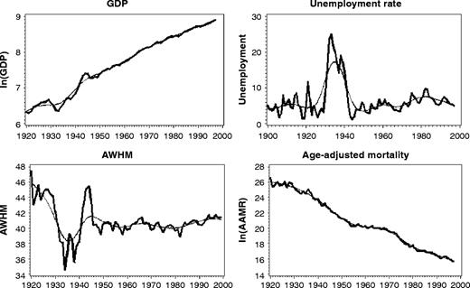
Four of the variables used in the study. GDP (in 1992 US$) and mortality are plotted in log scale. AWHM = average weekly hours in manufacturing. The thin line in each graph is a Hodrick–Prescott trend line (smoothing parameter = 100)
As early as the 1920s Dorothy Thomas found that economic expansions were associated with increases in mortality both in Great Britain and the US.1,2 This finding never received much attention, probably owing to its counterintuitive nature, in spite of being confirmed independently half a century later with US data by Eyer,3 Higgs,4 Graham et al.,5 and with Canadian data by Adams.6 Some of these authors referred to the association of increasing mortality with economic expansions as ‘perverse’.5
In the 1970s and 1980s, using Fourier analysis and time series models, Harvey Brenner and other authors tried to demonstrate lagged effects of the economy on mortality, with increases in mortality being produced by recessions occurring years before.7 These studies have generated controversy over the past two decades. In spite of its intuitive appeal, Brenner's models were considered unconvincing because of ad hoc use of detrending methods and lags, misspecification, and other statistical problems.8–13 More recently, Catalano14 claimed that while downward deviations from the trend in real gross national product per capita (i.e. recessions) have no effect on death rates, upward deviations (i.e. expansions) are associated with drops in age-standardized mortality one year later. This was interpreted as resulting from the loosening of governmental budgetary constraints during economic upturns, allowing for the expansion of health care to persons ‘not thought to be at sufficient risk to warrant attention at an earlier budget period’.14 This contribution by Catalano, who applied unconventional methods—like using Danish economic data as covariates in regression models for US mortality—has not been supported by recent work on the impact of economic fluctuations on mortality. Indeed the latest research10–12,15 supports the idea that mortality oscillates upwards during years of economic expansion and downwards during recessions.
The relationship between the economy and health remains a subject of controversy. Some of the literature relies on complicated statistical methods making the results difficult to interpret. In addition, the most recent analyses are limited to relatively short periods of two decades or less during the last quarter of the 20th century, but it is conceivable that this relationship could be different in different historical periods. In this paper I examine the relationship between economic fluctuation and mortality in the US throughout the 20th century with methods that are robust and simple. Since the impact of the economy on health may differ for different social groups, ages, and causes of deaths, differential effects on ethnic groups, age-and-sex strata and cause-specific mortality are also investigated.
Data and Methods
Data on mortality and economic indicators (Figure 1) were obtained from the Historical Statistics of the United States and other official sources (see Appendix for details). Since unemployment and real GDP (real gross domestic product, i.e. the volume of the national economy adjusted for inflation) are widely used to assess oscillations in the economy, they were chosen as economic indicators. Two other commonly used indicators of the business cycle—the index of manufacturing production, and the average of weekly hours in manufacturing16,17—were also investigated.
The foundation of the statistical methods used is the method of concomitant variation,18 a method to ascertain the relationship between two variables based on the fifth of John Stuart Mill's canons19 to establish causality—if two phenomena vary up and down simultaneously, one is causing the other or there is a third factor causing both of them. The deviations of an oscillatory variable with respect to its long-term trend, or its year-to-year rate of change, measure both the size and the direction of its change over time. Therefore, if two variables oscillate simultaneously, because one causes the other or a third factor causes both, their deviations from trend or their rates of change will be highly correlated.
In order to apply this method the variables were transformed either (i) into rates of change (i.e. the ratio (xt2xt21)/xt21 expressing the relative change from the former year); or (ii) into percentage deviation from trend, i.e. the ratio (xt2 xHP,t)/xHP,t where xHP,t is the trend value of the variable x at time t, computed with the Hodrick–Prescott filter (Figure 1), a widely used smoothing tool.20 The smoothing parameter was set to 100, a common option for annual data.
Correlations between the transformed variables were computed. In simple regression models the percentage change in mortality (for different population groups, time periods and seven causes of death) was regressed on GDP growth or the rate of change of unemployment to estimate the effect of changes in economic conditions on year-to-year variations in mortality. To examine if the effects changed or remained stable throughout the century (Figure 1), four periods of roughly similar length were analysed separately. Since several series are available only from 1920, the first period includes the years 1900–19 in which the fluctuations of the US economy were moderate, though it also includes the First World War. The next period, 1920–44, includes the years of accelerated economic growth in the 1920s, the protracted depressions of the 1930s and the Second World War. The third period, 1945–70, corresponds to the so-called golden age of the post-war US economy, with sustained GDP growth and weak increases of unemployment during recessions. The fourth period, from 1971 to the late 1990s, is characterized by stronger oscillations of unemployment and a reduction of GDP growth with respect to former years.
Results
There was no evidence of trends in the 10 series of transformed variables (age-adjusted mortality and the four economic indicators, in rates of change or percentage deviation from trend). The augmented Dickey–Fuller test rejected the hypothesis of unit roots (P < 0.001 in the 10 cases), indicating that the transformed series are trend-stationary.
Real GDP, manufacturing production and weekly hours in manufacturing grow (or are elevated over trend) during the economic expansions and contract (or are below trend) during recessions. Since these indicators oscillate simultaneously with the economy, their correlations rc as rates of change or rd as deviations from trend, are strongly positive (Table 1, columns A to F). In contrast, since unemployment grows when the economy contracts and drops when the economy expands (and is therefore referred to as a countercyclical indicator), its correlations rc and rd with GDP, manufacturing output and hours in manufacturing are strongly negative.
Correlations (Pearson coefficient, times 100) between four indicators of the US economy (real GDP, national unemployment rate, average weekly hours in manufacturing, and index of total industrial production) and age-adjusted mortality
| A | B | C | D | E | F | G | H | |||||||||
|---|---|---|---|---|---|---|---|---|---|---|---|---|---|---|---|---|
| Unemployment | Manufacturing hours | Industrial production | Age-adjusted mortality | |||||||||||||
| Period | rc | rd | rc | rd | rc | rd | rc | rd | ||||||||
| 1920–44 | ||||||||||||||||
| GDP | −74*** | −86*** | 69*** | 87*** | 81*** | 92*** | 36† | 41* | ||||||||
| Unemployment | −64*** | −79*** | −80*** | −89*** | −56** | −54*** | ||||||||||
| Manufacturing hours | 81*** | 88*** | 37† | 43* | ||||||||||||
| Industrial production | 52** | 57** | ||||||||||||||
| 1945–70 | ||||||||||||||||
| GDP | −87*** | −76*** | 90*** | 83*** | 83*** | 87*** | 48* | 20 | ||||||||
| Unemployment | −80*** | −58** | −88** | −69*** | −66*** | −46* | ||||||||||
| Manufacturing hours | 90*** | 80*** | 44* | 24 | ||||||||||||
| Industrial production | 49* | 31 | ||||||||||||||
| 1971–98 | ||||||||||||||||
| GDP | −88*** | −94*** | 71*** | 68*** | 87*** | 92*** | 36† | 37† | ||||||||
| Unemployment | −54** | −61** | −90*** | −93*** | −45* | −44* | ||||||||||
| Manufacturing hours | 66*** | 65*** | 45* | 45* | ||||||||||||
| Industrial production | 36† | 34† | ||||||||||||||
| 1920–99 | ||||||||||||||||
| GDP | −75*** | −84*** | 72*** | 86*** | 82*** | 92*** | 36** | 37** | ||||||||
| Unemployment | −66*** | −75*** | −80*** | −85*** | −56*** | −51*** | ||||||||||
| Manufacturing hours | 80*** | 86*** | 38*** | 40*** | ||||||||||||
| Industrial production | 49*** | 50*** | ||||||||||||||
Correlations computed with the variables transformed into annual rate of change (rc), or into percent deviation from a long-term trend (rd).
P < 0.10
P < 0.05
P < 0.01
P < 0.001.
Throughout the century and in each of the subperiods studied, the correlations rc and rd of age-adjusted mortality with GDP, manufacturing hours, and industrial production are positive, while the correlations of mortality with unemployment are negative (Table 1, columns G and H; Figure 2). This means that mortality rises when the level of economic activity accelerates and decreases when the economy slackens (rc); similarly, death rates are above the trend when ‘the economy’ is over the trend and below the trend when the economy is below the trend (rd). Therefore, mortality is what economists call a procyclical variable, oscillating up and down over its trend with the ups and downs of the economy.
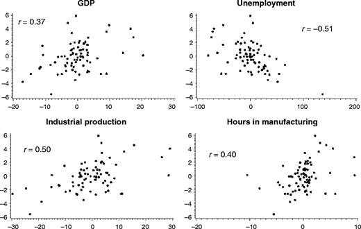
Age-adjusted mortality plotted against four economic indicators, USA 1920–1998. Variables in percent deviation from trend
For the whole period 1920–99 and all the subperiods considered, the statistically significant correlations of the four economic indicators with mortality have consistent signs (Table 1), suggesting that the results are robust to the business cycle indicator used. The identity of signs, and even the similarity of the values of the correlations for each pair of variables in rates of change (rc) and deviation from trend (rd) is strong evidence that these models are showing a real relationship between the oscillations of the series.
In simple regression models with the percentage change in mortality as the response variable regressed on an intercept and one economic indicator (GDP growth or the rate of change of unemployment), GDP growth is positively associated with percentage change in mortality, while the rate of change in unemployment is negatively associated with the percentage change in mortality (Table 2). The level of statistical significance is almost the same in GDP models and unemployment models, though slightly higher in the latter. In absolute value, the coefficient estimate for GDP effects is between 4 and 10 times larger than the estimate for unemployment. This is consistent with the fact that, throughout the century, the rate of change of unemployment oscillated within a range about 10 times larger than GDP growth.
Regression estimates of the year-to-year variation in the percentage change of age-adjusted mortality of the general population (A), whites (B), and non-whites (C) associated with a one percentage point increase in GDP growth or in the rate of change of unemployment
| Male | Female | Male and female | ||||||||||
|---|---|---|---|---|---|---|---|---|---|---|---|---|
| Period | GDP | Unemployment | GDP | Unemployment | GDP | Unemployment | ||||||
| (A) Age-adjusted mortality rate, total population | ||||||||||||
| 1900–19 | −0.053 | −0.039 | ||||||||||
| 1920–44 | 0.20† | −0.037** | 0.16 | −0.040** | 0.20† | −0.041** | ||||||
| 1945–70 | 0.25* | 20.038*** | 0.19* | 20.026* | 0.22* | 20.034*** | ||||||
| 1971–ca. 1996 | 0.18 | 20.033† | 0.19 | 20.048* | 0.27† | 20.048* | ||||||
| 1920–ca. 1996 | 0.20 | 20.020*** | 0.15* | 20.019*** | 0.19*** | 20.037*** | ||||||
| (B) Age-adjusted mortality rate, whites | ||||||||||||
| 1900–19 | −0.053 | −0.038 | ||||||||||
| 1920–44 | 0.20† | —0.039** | 0.17 | −0.042** | ||||||||
| 1945–70 | 0.27** | −0.038*** | 0.09 | −0.017† | ||||||||
| 1971–ca. 1996 | 0.10 | −0.030 | −0.13 | −0.010 | ||||||||
| 1920–ca. 1996 | 0.19*** | 20.037*** | 0.14† | 20.035*** | ||||||||
| (C) Age-adjusted mortality rate, blacks and other | ||||||||||||
| 1900–19 | −0.023 | −0.021 | ||||||||||
| 1920–44 | 0.27† | −0.034† | 0.21† | −0.030 | ||||||||
| 1945–70 | 0.37* | −0.056*** | 0.14 | −0.030* | ||||||||
| 1971–ca. 1996 | 0.25 | −0.050† | 0.44* | −0.088** | ||||||||
| 1920–ca. 1996 | 0.27*** | −0.039** | 0.20** | −0.034** | ||||||||
P < 0.1
P < 0.05
P < 0.01
P < 0.001.
The same general pattern—a positive association of mortality with GDP growth and a negative association of mortality with growth in unemployment—was observed but for a few exceptions across mortality of all ethnic groups (Table 2) age-and-sex strata (Table 3), and specific causes of death (Table 4). In all cases GDP effects were consistently several times larger in absolute value (on average, 6 times larger for cause-specific mortality, 9 times larger for age-and-sex specific mortality) and have opposite sign to those of unemployment, with a similar or slightly lower level of statistical significance. To save space these GDP effects are not reported for age strata, or for different causes of death.
Regression estimates of the year-to-year variation in the percentage change of sex-and-age-specific mortality associated with a one percentage point increase in the rate of change of unemployment
| Male | Female | |||
|---|---|---|---|---|
| (A) Under one year | ||||
| 1900–19 | −0.025 | −0.024 | ||
| 1920–44 | −0.030† | −0.035† | ||
| 1945–70 | 0.039 | 0.041 | ||
| 1971–ca. 1996 | −0.083** | −0.072* | ||
| 1900–ca. 1996 | −0.015 | −0.019 | ||
| (B) From 5 to 14 years | ||||
| 1900–19 | −0.087 | −0.024 | ||
| 1920–44 | −0.013 | −0.028 | ||
| 1945–70 | −0.063† | −0.041 | ||
| 1971–ca. 1996 | −0.086** | −0.079 | ||
| 1900–ca. 1996 | −0.032† | −0.040† | ||
| (C) From 15 to 24 years | ||||
| 1900–19 | −0.224 | −0.142 | ||
| 1920–44 | −0.063** | −0.040* | ||
| 1945–70 | −0.120*** | −0.068† | ||
| 1971–ca. 1996 | −0.061 | −0.070† | ||
| 1900–ca. 1996 | −0.099** | −0.061* | ||
| (D) From 25 to 34 years | ||||
| 1900–19 | −0.025 | −0.018 | ||
| 1920–44 | −0.054*** | −0.034* | ||
| 1945–70 | −0.084* | −0.056* | ||
| 1971–ca. 1996 | −0.056 | −0.047 | ||
| 1900–ca. 1996 | −0.103* | −0.075* | ||
| (E) From 35 to 44 years | ||||
| 1900–19 | −0.101 | −0.067 | ||
| 1920–44 | −0.045** | −0.041** | ||
| 1945–70 | −0.072*** | −0.059** | ||
| 1971–ca. 1996 | −0.050 | −0.059† | ||
| 1900–ca. 1996 | −0.057*** | −0.038*** | ||
| (F) From 55 to 64 years | ||||
| 1900–19 | −0.013 | −0.011 | ||
| 1920–44 | −0.026† | −0.027 | ||
| 1945–70 | −0.034** | −0.030** | ||
| 1971–ca. 1996 | −0.023 | −0.023 | ||
| 1900–ca. 1996 | −0.014* | −0.012* | ||
| (G) From 75 to 84 years | ||||
| 1900–19 | 0.002 | −0.002 | ||
| 1920–44 | −0.048* | −0.043** | ||
| 1945–70 | −0.025† | −0.029* | ||
| 1971–ca. 1996 | −0.020 | −0.044† | ||
| 1900–ca. 1996 | 20.034*** | 20.039*** | ||
P < 0.1
P < 0.05
P < 0.01
P < 0.001.
Regression estimates of the year-to-year variation in percentage change in mortality owing to seven major causes associated with a one percentage point increase in the rate of change of unemployment
| Period | Major CV diseasesa | Major CV and renal diseasesa | Cancer | Traffic injuries | Flu and pneumonia | Liver cirrhosis | Suicide |
|---|---|---|---|---|---|---|---|
| 1920–44 | −0.010† | 0.002 | 0.014 | −0.128* | −0.016† | 0.033† | |
| 1945–70 | −0.033** | −0.013* | −0.010b | −0.206** | −0.078** | 0.075** | |
| 1971–ca. 1996 | −0.038* | 0.006 | −0.174** | −0.105 | −0.061* | 0.047 | |
| 1920–ca. 1996 | 0.002 | 0.011 | −0.140*** | −0.019† | 0.037** |
P < 0.1
P < 0.05
P < 0.01
P < 0.001.
Historical statistics for cardiovascular (CV) disease mortality in the US are grouped with renal disease mortality until 1970.
This estimate of the percentage change in traffic mortality increases in absolute value to 20.112 (P < 0.001, R2 = 0.53) when the outlier years 1945–46 are excluded from the regression for the period 1945–70. Between 1945 and 1946 GDP contracted 11%, with unemployment jumping from 1.9 to 3.9%, and simultaneously traffic mortality increased 13%. All this was obviously related to the economic contraction and the return of US soldiers at the end of the Second World War.
For the regressions of mortality of the total population on unemployment (Table 2, panel A), R2 is 0.32 for the years 1920–96 and 0.43 for 1945–70. The R2 of the other regression models varied over a wide range (from as low as 0.01 for some cancer mortality regressions to as high as 0.53 for some traffic mortality models), but was always twice as big for regressions with unemployment as compared with those with GDP.
On average, age-adjusted mortality fell 1.35% per year during the period 1920–96, oscillating between a maximum annual reduction of 10.6% and a maximum annual increase of 6.3% (Figure 1). Thus the statistical association of the oscillations of mortality with those of the four economic indicators, shown in correlation (Table 1) and regression models (Tables 2–4), implies that the general decline in mortality accelerates during recessions and slows—or even reverses—during economic expansions.
Effects were larger for males than for females for the whole period and all the subperiods (Tables 2 and 3), except in 1971–96, when effects were either similar in both sexes or larger (in absolute value) for females than for males (Table 2, panels A to C). However, when sex differences in coefficients were tested,21 they did not achieve statistical significance, probably owing to reduced sample size.
There was some evidence that effects differed over time. Estimates for the earliest period (1900–20) have the same sign as estimates for the subsequent periods, but are almost always not statistically significant (Tables 2 and 3). Effect estimates (and statistical significance) often appear to increase from 1920–45 to the post-Second World War period. Indeed, it is in the period 1945–70 that the unemployment effect is the strongest for all male groups in the general population, including whites, non-whites (Table 2), all age groups from 15 to 64 (Table 3), and all causes of death (Table 4). However, for total mortality and total female mortality, the impact of economic fluctuations is strongest in the most recent period 1970–96 (Table 2, panel A). Unemployment effects (b ± SE[b]) intensified from 20.034 ± 0.008 in 1945–70 to 20.048 ± 0.002 in 1971–96 for total mortality (P = 0.14), and from 20.026 ± 0.010 in 1945–70 to 20.048 ± 0.022 in 1971–96 for female mortality (P = 0.18).
In the second half of the century, effects are substantially stronger for blacks and others than for whites. In 1971–96 the unemployment effect on mortality of non-white males (20.050 ± 0.024) is about twice that for white males (20.030 ± 0.019, P = 0.36) (Table 2, panels B and C). Effects are also significantly larger (P = 0.04) for non-white females (20.088 ± 0.026) than for white females mortality (20.010 ± 0.036).
Estimates of effects on age-specific mortality pooled over the whole period studied (1900–96) increase from the weakest effects on infant and child mortality to the strongest effects in teenagers and young adults aged 15–24 (Table 3). The effect progressively declines in older age strata, but increases again in the oldest age-group (people aged 74–84). However, in the years after 1970 strong effects emerge in children <1 year old, and aged 5–14. Indeed these are the only statistically significant effects on age-specific mortality in this period (the effect estimate is 20.089 ± 0.030 for children <1 year old, and 20.029 ± 0.016 for people aged 55–64 years, P = 0.09).
Analyses of cause-specific mortality (Table 4) indicate that economic expansion is positively—i.e. procyclically—associated with mortality for all causes of death investigated—major cardiovascular and renal diseases, cancer, traffic injuries, flu and pneumonia and liver cirrhosis—except suicide. For suicide, effects are in the opposite direction, with rates decreasing countercyclically when the economy expands. In all causes where comparison is possible, the largest effect is in the period 1945–70. Associations appear to be specially strong for traffic mortality in the second half of the century, as well as flu and pneumonia in the post-war years 1945–70. The impact of unemployment fluctuations on cancer mortality seems to be weak, though statistically significant in 1945–70 (20.013 ± 0.006), and disappears after 1970 (0.006 ± 0.010).
Discussion
The results of this study show that throughout the 20th century economic expansions in the US are associated with increasing mortality for all groups and causes of death studied, except suicide. Associations appear to be especially strong for traffic mortality after the mid-century, as well as flu and pneumonia in the post-war years 1945–70.
Any statistical association can be challenged as spurious by invoking confounders—or ‘omitted’ or ‘lurking’ or ‘third’ variables, in other jargons. In the models presented here the oscillations of four different economic indicators have significant associations with the oscillations of the death rate. Variables that might be confounding this association would have to be factors causing changes in mortality and statistically associated with the oscillations of the economy. Population-level variables like the annual volume of road traffic, the intensity of internal migration, or the average levels of immunity, ingestion of unhealthy substances, strength of social support or daily sleep, may have an effect on health and mortality, and they can also be associated with the oscillations of the economy as measured for instance by GDP growth or weekly hours of work, but are best thought of as mediators of the relationship between ‘the economy’ and mortality, rather than confounders. To understand concretely the relationship between economic fluctuations and changes in mortality these mediator variables will have to be studied for each particular cause of death.
Variables like weather, the position of the moon or particular planets or stars would be omitted variables confounding the association economy–mortality if it could be shown that oscillations of one of these variables modify both the condition of the economy and the level of mortality. In the late 19th century and early 20th century, economists like Stanley Jevons and Henry Ludwell Moore attributed business cycles to the influence of solar spots and weather, acting on agriculture.22 Though the cause of sequential expansions and contractions of the economy is one of the most obscure and contentious issues in economics, few economists would today defend any theory attributing recessions and expansions to weather or astronomical influences. It is unlikely that the associations reported here are owing to a third variable that causes both economic fluctuations and changes in mortality.
A common statistical problem in the analysis of time series data is autocorrelation. According to regression theory, autocorrelation of the residuals does not bias the regression estimates. However, positive autocorrelation reduces the standard error of the estimates while negative autocorrelation has the opposite effect, enlarging them.9 Autocorrelation of the residuals usually depends on autocorrelation of the response variable. In the present data the first order autocorrelations of the rates of change of age-adjusted and age-specific mortality were in the range −0.19 to −0.38. These autocorrelations are not large; moreover, they are negative, so if anything, they would have resulted in enlarged standard errors and spuriously reduced levels of statistical significance. In the regressions rendering statistically significant results, the Durbin–Watson d was generally not very far from 2.0 (indicating weak or no autocorrelation of the residuals) and there were no autocorrelation patterns in the plotted residuals. When some of the models were rerun with autocorrelated error correction using an autoregressive error model (instead the OLS estimates reported in the Tables 2–4), the coefficient estimates changed very little (though the d got closer to 2.0 and the level of statistical significance generally increased slightly). Therefore, on both theoretical and empirical grounds, spurious estimates owing to autocorrelation are not an issue in these analyses.
Statistically significant effects may be practically unimportant. Therefore it is important to place these patterns in the context of the observed changes in mortality and in the indicators of the US economy. During the period 1971–96, the effect of GDP growth on the rate of change of mortality of the general population (Table 2, panel A), is 0.274 ± 0.137, and the intercept estimate in that regression is 20.022 ± 0.005, therefore the rate of change in age-adjusted mortality, ã, will be ã = 20.022 + 0.274·g, where g is GDP growth. For ã = 0, g = 0.080 = 8.0%. Thus the model predicts that with GDP growing 8% annually, age-adjusted mortality will stay constant, while mortality will increase with GDP growth >8%, and will decrease with GDP growth <8%. For g = 0, ã = 20.022 = 22.2%. Mortality will drop 2.2% with a zero growth economy (a strong recession).
The largest expansion of the US economy after 1970 occurred in 1984, when GDP growth was 7.0%. The registered change in age-adjusted mortality that year was precisely 0.0%. Considering the period 1920–96 for which GDP data are available, the 5 years with the largest increases (all >3%) in age-adjusted mortality were 1923, 1926, 1928, 1936 and 1943, almost all of them years of strong GDP growth: 13.2, 6.6, 1.1, 13.1, and 16.3%, respectively (3 of these 5 years of high growth of mortality in 1920–96 are among the 5 years of highest GDP growth in the period). The 5 years with the worst recessions in terms of GDP contraction (between 23.6 and 213.3%) were 1930–32, 1938 and 1946. During these years mortality dropped between 1.6 and 6.8%. The largest drop in mortality between 1920 and the end of the century, 10.6%, was in 1921, a strong recession year during which GDP contracted 2.2%. Based on these examples, the changes in mortality described by these models seem therefore not only statistically significant but also public health relevant.
The correlations rc and rd between mortality and unemployment are greater in absolute value than those between mortality and the other three economic indicators (Table 1). The levels of statistical significance are also higher for the correlations mortality–unemployment than for the correlations of mortality with the other three economic indicators, and for the regression coefficients of unemployment compared with those of GDP, in the general mortality regressions (Table 2) and the regressions for mortality of specific age-and-sex strata or causes of death (corresponding to Tables 3 and 4, where only unemployment coefficients are shown). All this seems to suggest that unemployment is a better predictor of health fluctuations than other economic variables. Since GDP, unemployment, industrial production and manufacturing hours, though reflecting different aspects of the economy, fluctuate in parallel during expansions and recessions, they are highly correlated (Table 1) and therefore multiple regressions modelling mortality as a function of two or more of these four economic indicators (or others) produce unreliable results, owing to multicolinearity. When mortality was regressed simultaneously on two or more economic indicators, and an intercept, the signs of the estimates were the same to those obtained in two-variable regressions, but the only regressor still statistically significant was unemployment. This may result from multicolinearity, but the pattern of nullification of all the effects except that of the rate of change of unemployment in multivariate regressions is hard to interpret. From the point of view of population health, the rate of change of unemployment might be a better gauge of the economy than GDP growth or other economic indices, perhaps because unemployment is a better measure of the population-level consequences of economic expansions and recessions. In other investigations10–12,15 it has also been observed that regional GDP or income effects (that can be considered similar to GDP) on mortality are much more sensitive to specifications than regional unemployment effects.
In panel regressions with data for the states of the US in 1972–91 Ruhm10 obtained point estimates in the range 0.4–0.7% for the decrease in mortality associated with an increase of one percentage point in unemployment. From data of the German länder between 1980 and 2000 Neumayer12 estimated a larger effect of 21.1%, while in the present study, for the period 1971–96 in the US the size of the effect (see Appendix for details) is 22.2% (95% confidence interval (CI): 23.0 to 21.3%). The reasons for the differences in these estimates require further investigation.
Ruhm10,23 found a stronger impact of economic fluctuations on adult mortality and health in younger than in older ages which is consistent with the results of this study. Among the eight causes of death that he investigated, he also found the largest effects of the economy on traffic mortality, which is the cause of death most impacted by the economy among the seven specific causes of death studied here. The increase over the century in the effect of the economy on traffic mortality is easily explained by the emergence of traffic injuries as one of the major causes of death in the middle decades of the century. The increase of suicides when unemployment grows is consistent with a large body of literature.3,5,10,24 The fact that the impact of the economy on cancer mortality disappears after 1970 is consistent both with the findings of Eyer,3,25 and with Ruhm10 who did not find any impact of the economy on cancer mortality in the years 1972–91.
An increasing body of research13,26 shows that the parallel processes of the long-term decline in death rates and the long-term growth of the economy are not causally connected, because factors increasing the money value of economic output and factors improving health are generally different, and often opposite. Amartya Sen13 has found that during the 20th century, the decades of faster economic growth in Great Britain were also those of the slowest increase in expectancy of life, while decades of low growth of the economy were associated with more rapid increases of life expectancy. Brenner's model in which periods of recession have a lagged effect on health, increasing mortality 10–15 years later,7 has been questioned on several grounds.8,13,25,27 With the present data, when cross-correlations between the rate of change in an economic indicator and the rate of change in a death rate are computed, the highest cross-correlation is almost always at zero lag or at a short lag of 1 or 2 years. Similarly, in distributed lag regressions of mortality on the economic indicator including lags up to 25 years, coefficient estimates for the lagged covariate are almost always the highest at zero-lag and drop quickly when the lag increases (data not shown).
In panel regressions used in recent investigations of the impact of fluctuations of the economy on health10–12,15 data from a number of geographical units during a series of years are regressed on demographic and economic indicators and dummy variables for geographical units and years. Two advantages of panel studies over time series models are the larger sample size (increasing statistical power) and the simultaneous availability of cross-sectional and longitudinal data which may help avoid ‘omitted variable bias’ or ‘confounding’.
However, panel models with death rates as response variable also have drawbacks. Panels of death rates in levels have strong first order positive autocorrelation and heteroscedasticity (because the variance of a rate is inversely related to its denominator, and therefore varies widely across geographical units of different population size) that violate the assumptions of classical linear regression, requiring special methods (GLS or weighted regression) to adequately estimate standard errors. All this is not a significant problem with modern computational software but, conceptually, the models become quite complex when these are combined with others such as the possible presence of region-specific time trends in the dependent variable.10–12,15 It is often difficult to choose among a variety of possible specifications and the choice of specification may have important consequences for the effect estimates obtained. The methods used in this study (with variables in rates of change or deviation from trend) are simpler than panel regressions (with variables in levels), but render similar results.
Many mechanisms may be responsible for the procyclical oscillation of mortality. Work pace, work time, and overtime increase during economic expansions.16,17 Economic upturns are also associated with rising levels of alcohol and tobacco consumption, overweight and obesity, decreased levels of exercising,23,28 reduced levels of sleep,29 and drops in time and opportunity for social interactions—with the consequent deterioration of social support. These mechanisms could be related to mortality through a variety of pathways including the direct effects of alcohol and smoking, increased levels of industry-related and traffic-related atmospheric pollution, possible stress-related30–33 effects on immunity and infectious disease (including microepidemics), and other processes leading to the precipitation of death in persons with underlying chronic disease. Moreover, during business expansions high work-pace and increasing business-related and recreational traffic raise the incidence of industrial injuries and traffic fatalities. Many of these pathways, obviously compatible with the results of this study (Table 4), were already proposed long ago by Joseph Eyer.25,27 In the US heart attacks in working individuals peak on Mondays10 and during the first week of the month there is a significant increase of deaths by external causes, circulatory disorders, cancer and other causes.34 In Israel, Sunday is the day of the week when there are more deaths among Jews—among Arabs there is no clear pattern.35 These patterns not only prove that death is a social event, but also that its concrete timing, even when it is owing to chronic diseases, is subject to influences that have a very short lag.
The observed larger impact of economic fluctuations in women and non-whites in recent decades may reflect the fact that changes in working and living conditions associated with the business cycle are more intense in these groups, formerly less integrated in labour markets, now more frequently hired for low-quality jobs and more often exposed to poor working conditions both in terms of work environment and job stability. Given the large proportion of childhood deaths in the US owing to unintentional injuries, it may be speculated that the large impact of economic expansions on children in the period 1971–96 could be related to the combined impact of lack of appropriate day care and overworked parents unable to provide appropriate care for their offspring.
The present investigation is an ecological study showing a detrimental effect of economic expansions on the health (as indexed by mortality) of the US population as a whole and particularly, in recent decades, of non-whites, and women. These results are not incompatible with those of studies in individuals showing an association between individual unemployment and bad health. However, the results of this study largely question the frequently made inference that, if joblessness has detrimental effects on the health of the jobless person, decreasing unemployment in an expanding economy must translate into improving health and decreasing mortality for the population as a whole. The presence of this relationship raises important and complex questions for policy, the discussion of which is beyond the scope of this article.
Appendix
Data sources and some statistical issues
Most data through 1970 used in this paper are taken from Historical Statistics of the United States. Time series have been extended until the second half of the 1990s with data from several issues of Vital Statistics of the United States, the Statistical Abstract of the US, the Economic Report to the President, and online historical statistics of the Bureau of Labor Statistics (series CEU3000000005 and LNS14000000) and the Federal Reserve (Historical Data series B50001). Real GDP data for the period 1929–98 in chained 1992 dollars are taken from Statistical Abstract of the United States 1999. GDP data for 1920–28 were obtained by conversion of GDP in 1929 dollars taken from Historical Statistics of the United States (conversion factor, 7.63). Since the rate of change or rate of growth of inflation-adjusted GDP is usually abridged to ‘GDP growth’, that term has been used in the text.
Except those for major cardiovascular disease in 1971–96, results for cause-specific mortality rates in Table 4 are not adjusted for age. However, the short-term oscillations that are captured by the rate of change of the mortality rate are likely to be very similar for crude and age-adjusted cause-specific mortality, since changes in the age-structure of the population may displace the long-term path of age-adjusted mortality but are unlikely to impact its short-term oscillations. For the period 1970–96 both age-adjusted and crude mortality owing to major cardiovascular diseases were available. Regressing the rates of change of these two series on GDP growth, the coefficient estimates for the GDP effect were 0.144 and 0.145. However, the level of statistical significance for the effect estimate from regression with age-adjusted mortality was much higher (P = 0.04) than that of the estimate from the regression with crude mortality (P = 0.34). Comparing the coefficient estimates of the effect of an economic indicator on the rate of change of age-adjusted and crude total mortality, the coefficient estimates for the whole period 1920–96 and the three subperiods differ by <10%, with the level of statistical significance slightly higher for the coefficient estimates derived from regressions with age-adjusted mortality. So Table 4 estimates from regressions with age-adjusted cause-specific mortality would probably be very similar in size but with higher levels of statistical significance.
Let ũ and ã be the rates of change of unemployment and age-adjusted mortality, respectively, so that ũ = (ut2 ut21)/ut21 = Du/u, and ã = (at2 at21)/at21 = Da/a, where ut and at are the unemployment and age-adjusted mortality at the year t, respectively, and Du and Da the change in u or a, respectively, from the year t − 1 to the year t. In the univariate regression to estimate the effect of ũ on ã the coefficient estimate for ũ is −0.048 ± 0.018 (Table 2, panel A), and the intercept estimate is −0.014 ± 0.003. Therefore, ã = −0.014 × 0.048·ũ < and Da/a = −0.014 − 0.048 Du/u. Assuming an annual absolute increase of one percentage point in unemployment (Du = 1) starting from an unemployment u at the average level during the period (u = 6.3) we have that Da/a = −0.014 −0.048/6.3 = −0.022 = −2.2%. The model predicts an increase of a one percentage point in unemployment associated on average with a decrease of 2.2% in age-adjusted mortality. The 95% CI, −3.0 to −1.3%, has been computed with SAS (PROC REG, MODEL option CLM).
This work largely benefited from comments and criticism of anonymous reviewers. Ana Diez Roux greatly helped with comments and editing.
References
Ogburn WF, Thomas DS. The influence of the business cycle on certain social conditions.
Higgs R. Cycles and trends of mortality in 18 large American cities,
Jin RL, Chandrakant PS, Svovoda TJ. The impact of unemployment on health: a review of the evidence.
Brenner MH. Political economy and health. In: Amick III BC, Levine S, Tarlov AR, Walsh DC, eds. Society and Health. New York: Oxford University Press,
Kasl S. Mortality and the business cycle: some questions about research strategies when utilizing macro-social and ecological data.
Søgaard J. Econometric critique of the economic change model of mortality.
Gertham U-G, Ruhm C. Death rise in good economic times: evidence from the OECD. NBER Working Paper Series No. 9357. Cambridge, MA: National Bureau of Economic Research,
Neumayer E. Recessions lower (some) mortality rates: evidence from Germany.
Sen A. Economic progress and health. In: Leon DA, Walt G, Walt G (eds). Poverty, Inequality and Health: An International Perspective. New York: Oxford University Press,
Catalano R. The effect of deviations from trend in national income on mortality: the Danish and USA data revisited.
Tapia Granados JA. Mortality and economic fluctuations—Theories and empirical results from Spain and Sweden. PhD Dissertation, Chapter 2, Department of Economics, Graduate Faculty of Political and Social Science, New School University, New York,
Zarnowitz V. Indicators. In: Eatwell J, Milgate M, Newman O (eds). The New Palgrave—A Dictionary of Economics. Vol. 2. London: Macmillan,
Mill's canons. In: Last J (ed.) A Dictionary of Epidemiology, 4th edn. New York: Oxford University Press,
Mill JS. A System of Logic, Ratiocinating and Inductive: Being a Connected View of The Principles of Evidence and The Methods of Scientific Investigation. 8th edn. New York: Harper & Brothers,
Backus DK, Kehoe PJ. International evidence on the historical properties of business cycles.
Clogg CC, Petkova E, Haritou A. Statistical methods for comparing regression coefficients between models.
Ruhm CJ. Healthy living in hard times. NBER Working Paper Series No. 9468. Cambridge, MA: National Bureau of Economic Research,
Eyer J. Does unemployment cause the death rate peak in each business cycle?
Easterlin RA. How beneficent is the market? A look at the modern history of mortality.
Eyer J. Capitalism, health, and illness. In: McKinlay JB. Issues in the Political Economy of Health Care. New York: Tavistock,
Kalimo R, El-Batawi MA, Cooper CL (eds). Psychosocial Factors at Work and their Relation to Health. Geneva: WHO,
Sparks K, Cooper C, Fried Y, Shirom A. The effects of hours of work on health: a meta-analytic review.
Sokejima S, Kagamimori S. Working hours as a risk factor for acute myocardial infarction in Japan: a case-control study.
Kiecolt-Glaser JK, McGuire L, Robles TF, Glaser R. Emotions, morbidity, and mortality: new perspectives from psychoneuroimmunology.
Phillips DP, Christenfeld N, Ryan NM. An increase in the number of deaths in the US in the first week of the month.

